U.S. cities offer different amenities, wage levels, and costs of living. One might expect that a combination of good amenities, high wages, and a low cost of living would make a city grow over time, attracting people from other areas and reducing outflow. One might also expect that a city with poor amenities, depressed labor markets or wages, and a high cost of living would lose population over time. In this essay, we briefly review whether this simple theory appears to describe the real world. To do so we analyze population growth and the real (i.e., price-level adjusted) income of the largest U.S. metropolitan statistical areas (MSAs) over the past 45 years. 

Recently, the Bureau of Economic Analysis (BEA) published for the first time data on regional price parities (RPPs), which express regional price levels as a percentage of the overall national price level for a given year. A price level is the average price paid by consumers for a mix of goods and services; that is, it describes the purchasing power of a dollar. RPPs, then, allow for the comparison of costs of living among MSAs. Intuitively, we know that a dollar can buy more in Nebraska than in California, even though wages are also higher in California than in Nebraska. Thus, RPPs allow us to compare real wages—that is, how much workers can buy in different MSAs.

A related concept also from the BEA is that of implicit regional price deflators (IRPDs), which measure regional price levels. While RPPs capture how prices vary across MSAs at one point in time, IRPDs capture differences in purchasing the same basket of goods both across locations and over time.¹ Real income differences across MSAs could be the result of differences in nominal income or in the cost of living across cities.

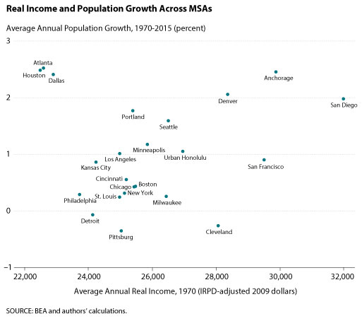
We want to know whether higher average real income in an MSA is correlated with higher population growth in that region. It could be that higher population growth is the result of both higher inflows of people into the city and lower outflows. The figure plots each selected MSA's average real income in 1970 relative to population growth over the next 45 years, 1970-2015. 

The figure seems to indicate a positive correlation between these variables. For instance, the Seattle, Denver, Anchorage, and San Diego MSAs, which had relatively higher real incomes in 1970, experienced high population growth over the period. On the other hand, the Detroit, Philadelphia, and Pittsburgh MSAs, which had lower real incomes in 1970, seem to have experienced lower (negative) population growth. Not all cities exhibit the positive correlation, however. The Atlanta, Houston, and Dallas MSAs had low average real incomes in 1970 yet experienced high population growth over the period. Incomes in these MSAs, however, have grown rapidly since 1970, which could be a main reason for the population growth.

In addition, factors other than real income in the early 1970s could be related to population growth—for example, amenities (not discussed here), which may have changed over time. That is, all else equal, some places are more desirable to live in than others. The link between an area's average real income and subsequent population growth, however, suggests that areas with currently high average real incomes will experience higher population growth in the coming years.

Note

¹ The data on RPPs, IRPDs, and real income start in 2008. To study the long-term trends in real income, we extend the IRPD series back to 1970. To do so we use consumer price index data for the largest MSAs going back to 1970 and combine it with the IRPDs. Data on average nominal income for the largest MSAs are available for the given time period. We compute average real income as the ratio of the nominal income to our constructed IRPD for an MSA in a given year. When we compare the real income generated from our computations and the one from the BEA for 2010, we find that the correlation between the two measures is quite high, 0.9813. This high correlation suggests that our method of extending IRPDs back in time should lead to a good approximation.

© 2017, Federal Reserve Bank of St. Louis. The views expressed are those of the author(s) and do not necessarily reflect official positions of the Federal Reserve Bank of St. Louis or the Federal Reserve System.